Visualizing Mode Connectivity
Blogpost by Pavel Izmailov, Timur Garipov and Andrew Gordon Wilson; visualizations in collaboration Javier Ideami.
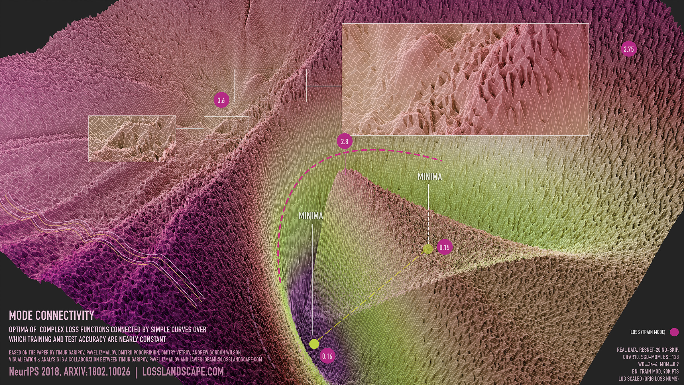
Figure 1: visualization of mode connectivity for ResNet-20 with no skip connections on CIFAR-10 dataset. The visualization is created in collaboration with Javier Ideami (https://losslandscape.com/).
Understanding generalization in deep neural networks is a great open question. Neural networks are trained by minimizing loss surfaces that are highly multimodal, with many settings of parameters that achieve no training loss but poor generalization. By understanding the geometric properties of these loss surfaces we can begin to resolve these questions and build more effective training procedures. Indeed, the local smoothness and convexity of loss surfaces is used for analyzing convergence of SGD and other optimizers [e. g. 12]. Recently, stochastic weight averaging [5] was proposed to find flatter regions of the loss, leading to better generalization.
The shape of the surface also has great implications for Bayesian approaches in deep learning. With a Bayesian approach, we not only want to find a single point that optimizes a risk, but rather to integrate over a loss surface to form a Bayesian model average. The geometric properties of the loss surface, rather than the specific locations of optima, therefore greatly influences the predictive distribution in a Bayesian procedure. Accordingly, recent approaches have exploited the geometry of the SGD trajectory for scalable and high performing Bayesian inference procedures [6, 7].
We still know very little about the properties of these loss surfaces. New discoveries are being made, showing topological behaviour that is highly distinct to neural networks. In this blogpost we describe mode connectivity, a surprising property of modern neural net loss landscapes presented in our NeurIPS 2018 paper. Our exposition in this post focuses on obtaining intuition through visualization.
Typically, the local optima of deep neural networks are imagined as isolated basins, as in the left panel of Figure 2. In this figure, we visualize the high dimensional loss surface in the plane formed from all affine combinations of three independently trained networks. In the next section we describe the details of the visualization procedure. This intuition comes from the following experiment: if we train two networks of the same architecture, we get two different local optima in the parameter space; the loss along the line segment connecting the two solutions blows up between the optima, reaching values attained by completely untrained networks at initialization. Surprisingly, the optima are actually not isolated. We can find a curved path between them, such that the loss is effectively constant along the path. We refer to this phenomenon as mode connectivity. These curved paths can be very simple, such as those shown in the middle and right panels of Figure 2. These paths are also easy to find, as we explain below.
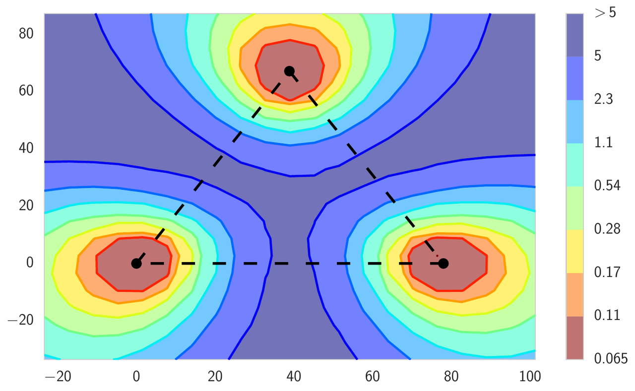
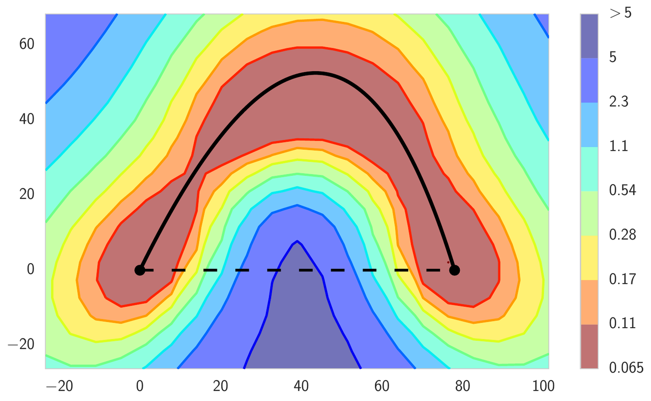
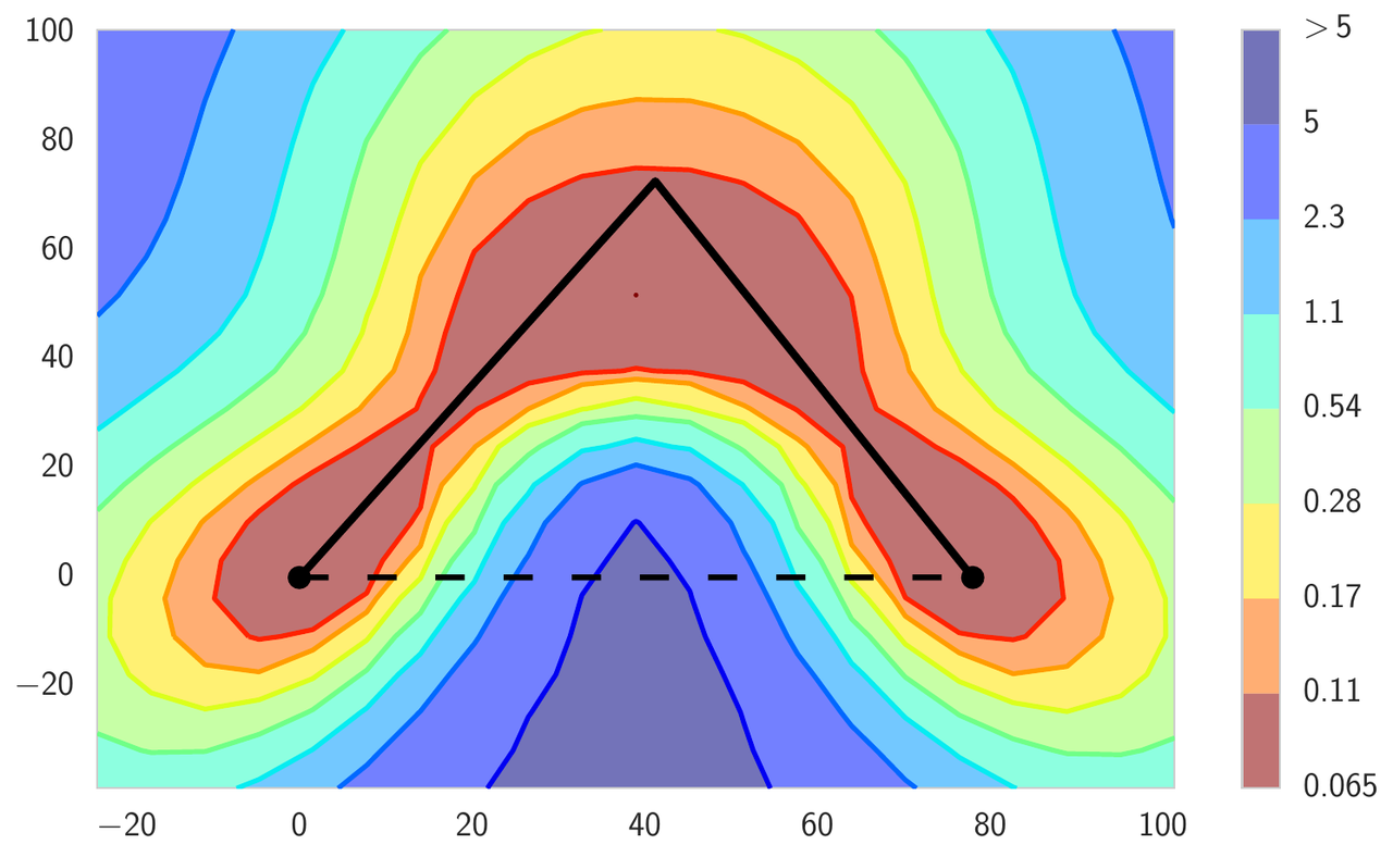
Figure 2: Loss surface of ResNet-164 on CIFAR-100. Left: three optima for independently trained networks; Middle and Right: A quadratic Bezier curve, and a polygonal chain with one bend, connecting the lower two optima on the left panel along a path of near-constant loss.
Mode connectivity has been shown to hold very generally. In [1, 2] mode connectivity is demonstrated for multiple state-of-the-art image classification architectures and some recurrent architectures on text data. In [3] the authors show that it is possible to connect optima trained with different optimizers and hyper-parameters, such as batch sizes, weight decay, learning rate schedule and data augmentation strategy. In [4] the authors that mode connectivity holds for policy optimization algorithms in deep reinforcement learning.
How to Visualize Loss Surfaces?
Visualization helps us analyze and build intuition about complex objects. Visualizations based on dimensionality reduction can reveal interpretable structure, leading to new scientific insights; for example, in [11] t-SNE visualizations were used to discover new sub-types of retinal cells. Here, we study the properties of loss functions of deep neural networks, which depend on millions (or sometimes even billions!) of parameters. We cannot directly visualize a million-dimensional surface. However, we can look at a 2D slice of the loss function, and if this slice is chosen carefully, it can provide insights about the structure of the landscape.
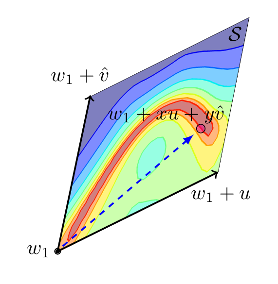
Figure 3: Illustration of the loss surface visualization procedure. We pick a 2D plane in the parameter space of a neural network, construct a coordinate system in the plane and define a grid in this coordinate system. Then, we evaluate loss for each point in the grid and visualize the result.
Three points in the parameter space always define a unique 2D plane that passes through these points. Suppose we have three points \(w_1, w_2, w_3\) in the weight space. These can, for example, be the vectors of parameters (all weights and biases concatenated into a single vector) of three independently trained networks, as in the left panel of Figure 2. We can construct a 2-dimensional plane passing through \(w_1, w_2, w_3\) as follows. We define a basis for the plane to be \(u = (w_2-w_1), v = (w_3-w_1)\) and the shift vector to be \(w_1\). We can orthogonalize the basis by switching to \(v=v - cos(u, v) u\), where \(cos(u, v)\) is the cosine of the angle between vectors \(u\) and \(v\). We can then define a Cartesian coordinate system in the plane and map \((x, y)\) coordinates to the points in the original parameter space using the formula \(w(x, y) = w_1 + u\cdot x + v\cdot y\). Now we can construct a grid in the coordinate system and evaluate the loss function for the network corresponding to each of the points in the grid, and visualize the results. Figure 3 illustrates the visualization process.
Finding Paths between Modes
The method for finding a path of low loss between a pair of optima is intuitively very simple: we parameterize the path and minimize the average loss along the path with respect to its parameters. Formally, suppose we have two optima \(w_1\) and \(w_2\) of the loss function. We then define a path connecting them as \(\phi(t)\), a mapping from the segment \([0, 1]\) to the parameter space, such that \(\phi(0) = w_1, \phi(1) = w_2\). For example, we can use a quadratic Bezier curve: \(\phi(t) = (1 - t)^2 w_1 + 2t (1-t) \theta + t^2 w_2\), shown with a black line in the middle panel of Figure 2. Here is the parameter of the curve, which has the same dimensionality and structure as the weight vectors \(w_1\) and \(w_2\). We train to minimize the average loss over the curve. Specifically, we minimize
with respect to \(\theta\), where \(Loss()\) is the standard loss function used for training the networks \(w_1\), \(w_2\), such as cross-entropy loss for classification.
We can compute stochastic gradients of \(L(\theta)\) with respect to \(\theta\) efficiently. To do so, we sample a point \(t\) uniformly on \([0, 1]\), and then compute the gradient of \(Loss(\phi(t))\) with respect to \(\theta\) using the chain rule:
Using this stochastic gradient estimate, we minimize \(L(\theta)\) with standard SGD.
For the quadratic Bezier curve, the whole path \(\phi(t)\) lies in a 2-dimensional subspace of the parameter space. We can visualize the loss function in this plane throughout training, using the visualization procedure described in the previous section.
High-Resolution Visualizations of Mode Connectivity
In collaboration with Javier Ideami we have recently produced high-resolution visualizations of the loss surfaces in the planes containing mode connectivity. We created a video showing the training process of a quadratic Bezier curve connecting a pair of local optima for ResNet-20 with no skip connections on CIFAR-10:
In the video, the optima go from being isolated and disconnected for the randomly initialized curve to being connected by a tunnel of low loss, as in Figure 1.
We have also created static visualizations of ResNet-20 on the FastAI Imagenette dataset at an even higher resolution of 1000x1000. We show these visualizations in Figures 4, 5, 6.
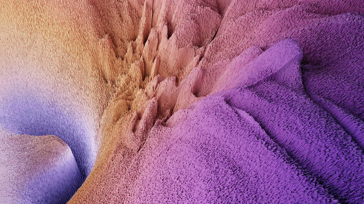
Figure 4: Visualization of mode connectivity for ResNet-20 with no skip connections on ImageNet dataset. The visualization is created in collaboration with Javier Ideami (https://losslandscape.com/).
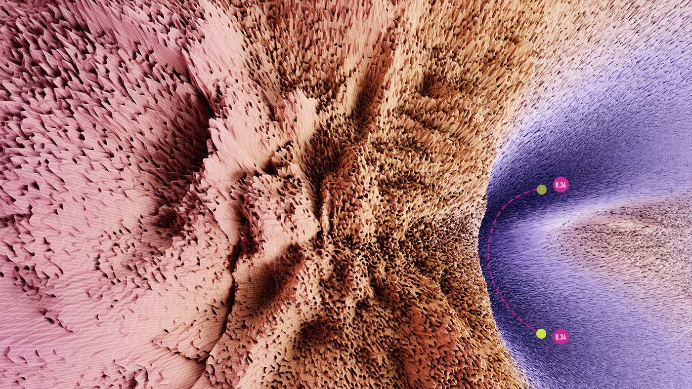
Figure 5: visualization of mode connectivity for ResNet-20 with no skip connections on Imagenette dataset. The visualization is created in collaboration with Javier Ideami (https://losslandscape.com/).
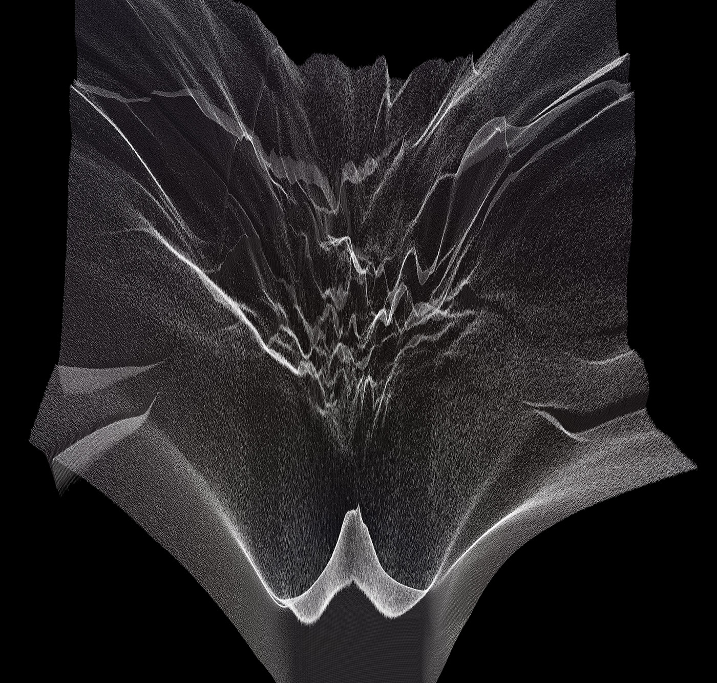
Figure 6: visualization of mode connectivity for ResNet-20 with no skip connections on Imagenette dataset. The visualization is created in collaboration with Javier Ideami (https://losslandscape.com/).
On Javier’s website https://losslandscape.com/ you can find other artistic high resolution visualizations of neural network loss surfaces, both static and dynamic.
Computational Cost of Creating the Visualizations
For each of the visualizations we compute the loss for each point in a grid (corresponding to a different setting of network weights). For Figures 4, 5, 6 we used a 1000x1000 grid, which requires evaluating the loss for a neural network at a million different settings of its parameters. For the video we computed 600 frames at a resolution of 300x300, amounting to over 50 millions loss evaluations. In order to limit the computational cost, we use a subsampled version of the dataset, making sure that this subsampling preserves the structure in visualizations. Even with the smaller dataset, the visualization process for the video took over two weeks using 15 GPUs. Creating the high-resolution static visualizations in Figures 4, 5, 6 took about two days using three GPUs.
Do These Paths Contain Different Representations?
The parameterization of neural networks is known to contain degeneracies. For example, in ReLU networks we can multiply the weights in one layer by a certain value, and divide the weights in the next layer by the same value, and the outputs of the network (and consequently loss) wouldn’t change. It is thus natural to ask whether the mode connectivity only exists because of such degeneracies in parameterization. We find, instead, that the low loss paths contain a rich collection of different representations, providing different predictions on test data. We demonstrate the diversity of functions along a path of low loss for a 1D regression problem in Figure 7.
Figure 7: Loss surface in the 2D plane containing a path of low loss (right) and the predictive functions corresponding to different points in this plane (left) for a DNN trained on a 1D regression problem. Different points along the curve shown with magenta circles on the right correspond to different functions shown with magenta lines on the left. Please see [7] for a detailed description of this experiment.
Indeed, the curves connect a pair of different optima \(w_1\) and \(w_2\), which produce different predictions. Therefore the predictions must change in some way along the curve. We can verify that the predictions of the networks along the path \(\phi\) are meaningfully different by looking at the performance of ensembles of these networks. We consider ensembles of two networks: one is fixed at \(w_1\) and the other \(\phi(t)\) is moving towards \(w_2\) along the path \(\phi\). We find that the ensemble of \(w_1\) and \(\phi(t)\) performs as well as the ensemble of independently trained \(w_1\) and \(w_2\) even for \(t \approx 0.3\), suggesting that the networks along the path are meaningfully different from the endpoints. We visualize the performance of the ensemble as a function of the point on the curve in Figure 8.
Figure 8: Performance of the ensemble of an endpoint of the path and a point on the path as a function of the point on the path. For comparison we visualize the ensemble performance for the direct line segment connecting optima, as well as for the path learned by our method.
New Work
There are several papers that provide theoretical explanations of mode connectivity. For example, the recent paper [4] demonstrates that different notions of noise stability, such as stability to dropout perturbations, imply mode connectivity. Papers [8, 9] provide different theoretical perspectives on mode connectivity by showing that under certain assumptions all sublevel sets of DNN loss are connected.
Mode connectivity inspired new practical methods for training neural networks with improved generalization and uncertainty quantification. At a high level, mode connectivity shows it is possible to travel between different modes of the loss function without leaving a general region of low loss. Stochastic Weight Averaging (SWA) [5] uses this idea and explores diverse solutions around a given solution by running SGD with a high constant learning rate; then, SGD iterates from different epochs are averaged to get a new solution with significantly improved generalization. SWA-Gaussian [6] extends SWA to also capture the covariance of SGD iterates and constructs a Gaussian distribution over the weights; by sampling from this distribution to form a Bayesian model average it is possible to significantly improve both the accuracy of the model and uncertainty representation, compared to standard SGD. Finally, [7] approximates the Bayesian posterior over the weights of a network in the subspace containing a path of low loss between optima and performs Bayesian model averaging using this approximation.
The recent paper [10] extends our method for finding low loss curves, to find planes where the loss surface resembles a given picture. Surprisingly, they were able to find such planes for any picture they used. We show some of their example loss surfaces in Figure 9. The fact that simple SGD can easily find these complex structures in the loss surface hints at a blessing of dimensionality. The high dimensionality of the parameter space provides many paths towards good solutions.
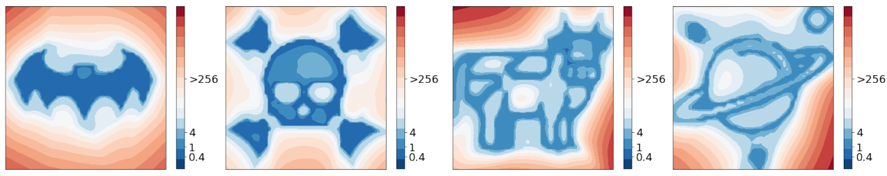
Figure 9: visualization of the loss in planes constructed in [10] for FashionMNIST and CIFAR-10 datasets. This figure is copied directly from [10].
References
[1] Loss Surfaces, Mode Connectivity, and Fast Ensembling of DNNs; Timur Garipov, Pavel Izmailov, Dmitry Podoprikhin, Dmitry Vetrov, Andrew Gordon Wilson; Neural Information Processing Systems (NeurIPS), 2018
[2] Essentially No Barriers in Neural Network Energy Landscape; Felix Draxler, Kambis Veschgini, Manfred Salmhofer, Fred A. Hamprecht; International Conference on Machine Learning (ICML), 2018.
[3] A Closer Look at Deep Learning Heuristics: Learning rate restarts, Warmup and Distillation; A. Gotmare, N. Keskar, C. Xiong & R. Socher; International Conference on Learning Representations (ICLR) 2019
[4] Understanding the impact of entropy on policy optimization; Zafarali Ahmed, Nicolas Le Roux, Mohammad Norouzi, Dale Schuurmans; International Conference on Learning Representations (ICLR) 2019
[4] Explaining Landscape Connectivity of Low-cost Solutions for Multilayer Nets; Rohith Kuditipudi, Xiang Wang, Holden Lee, Yi Zhang, Zhiyuan Li, Wei Hu, Rong Ge, Sanjeev Arora; Neural Information Processing Systems (NeurIPS), 2019
[5] Averaging Weights Leads to Wider Optima and Better Generalization; Pavel Izmailov, Dmitry Podoprikhin, Timur Garipov, Dmitry Vetrov, Andrew Gordon Wilson; Uncertainty in Artificial Intelligence (UAI), 2018
[6] A Simple Baseline for Bayesian Uncertainty in Deep Learning Wesley Maddox, Timur Garipov, Pavel Izmailov, Dmitry Vetrov, Andrew Gordon Wilson Neural Information Processing Systems (NeurIPS), 2019
[7] Subspace Inference for Bayesian Deep Learning; Pavel Izmailov, Wesley J. Maddox, Polina Kirichenko, Timur Garipov, Dmitry Vetrov, Andrew Gordon Wilson; Uncertainty in Artificial Intelligence (UAI), 2019
[8] On Connected Sublevel Sets in Deep Learning; Quynh Nguyen; International Conference on Machine Learning (ICML), 2018.
[9] Topology and Geometry of Half-Rectified Network Optimization; C. Daniel Freeman, Joan Bruna
[10] Loss Landscape Sightseeing with Multi-Point Optimization; Ivan Skorokhodov, Mikhail Burtsev, 2019
[11] Highly Parallel Genome-wide Expression Profiling of Individual Cells Using Nanoliter Droplets